Statistics

Using Python to Calculate Dice Statistics

March 19, 2019

NOTE: This post was originally created as a lesson for my AP high school students. The target audience is proficient beginners with at least 1 year of programming experience and some math pre-reqs.

Every time I visited Las Vegas as a young kid, I would get kicked out of the casinos. I just wanted to play the games. But rules are rules, and I had to wait until I was 21.

When I was finally of age, a few friends and I hopped in my car and drove the 4.5 hours from Los Angeles to Sin City. We checked into our hotel and I was immediately hooked. It was at that moment, that I understood how people descend into addiction. Few feelings are like the hit of dopamine you receive when you score big on the craps table.

And yes, my game is craps. That first weekend one of our good friends had a 45 min hot streak where he rolled only a single 7. Everyone won a ton of money and we all went nuts. Anyone who’s played before knows how rare a streak like that is, but at the time I had no idea. In the visits that followed I pretty much lost money every time. Factor in how much I enjoyed each experience and I’d like to believe I’ve broken even in the long run.

Today I’m only slightly older and barely wiser, but I have taken a statistics course recently. And now I have a much better grasp on the actual numbers behind how likely I am to win each roll.

In this post, we’ll write some code that performs some simple calculations on the probability of different dice rolls.

If you want to follow along with the post, here’s a colab notebook that will get you going.

We’ll start with a quick detour and then explore the statistics inherent to dice rolling. In the pursuit of that goal, we’ll use python to simulate this process experimentally.

First, Let’s Play a Game

Two of my students, Xochitl and Jimmie, play a game where each takes a turn rolling two six-side dice.

Xochitl gets $1 if the sum of the numbers of the two dice is a prime number (the number 1 is not prime).

Jimmie gets $2 if the numbers on the two dice are the same (e.g. 1-1, 2-2, 3-3, etc).

Who makes more money on average?

Let’s write some python and figure it out.

We start by loading in a few python specific libraries on lines 1, 2, and 3. We’ll use matplotlib and seaborn for plotting, and numpy for data processing.

Then we add a bit of setup to our plotting on lines 5 and 6.

Next, we set a random seed for numpy on line 8 to make sure that our results are reproducible (randomness in computers is pretty dicey - pun intended - so we use the pseudo-randomness that comes with numpy).

On lines 10 and 11, we create numpy arrays that hold the sample space for our two dice.

Line 13, 14, and 15 hold python lists where we’ll store the outcomes for each of the two dice, and their sum.

Finally, we loop $500$ times, picking a random number from the sample space for each dice and appending them to their respective arrays. We also append their sums, and call it a day.

After running this code, we should be able to plot the results. Here’s the code:

And here’s what we get:

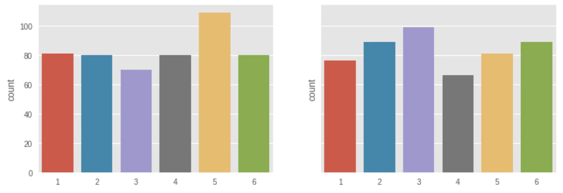
Interesting. Looks like 500 rolls doesn’t give us consistent results for our dice rolls. Die #1 rolled $5$ significantly more times than die #2, among other identifiable differences.

Let’s look at their sums.

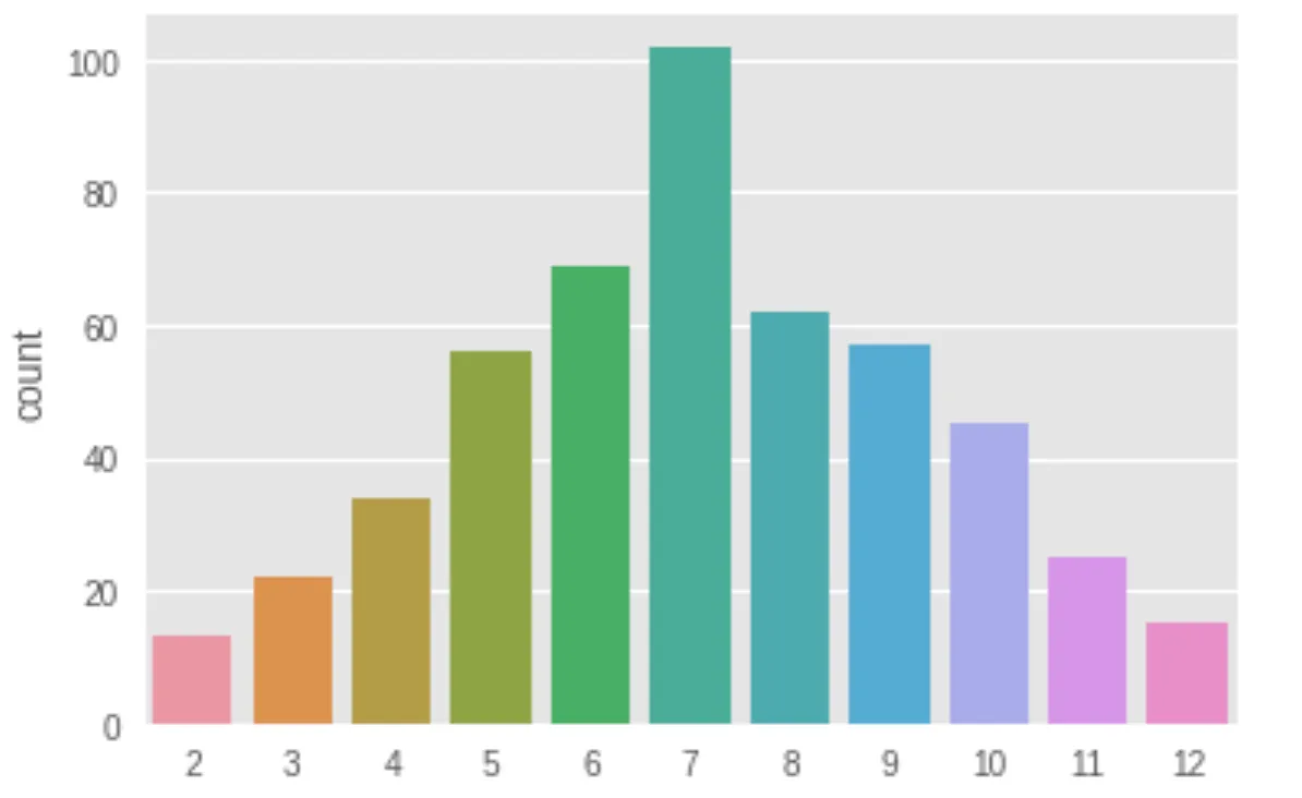
This shows a clear sign. Sevens got rolled the most.

The Law of Large Numbers

Now we didn’t get results consistent with what we know to be true. For any fair dice, every number is equally likely to be rolled. However, we see clear discrepancies in our results because we only ran the trials $500$ times. If we up that number to $5,000$ or $10,000$, we’ll start to see our outcomes converge to their expected values. This is due to the law of large numbers, which states that as the number of samples increases, their respective probabilities converge to their true probabilities.

Let’s re-run our experiment with 20x more trials and see how our results look.

The only thing that’s changed is on line 9. We’ve replaced $500$ with $10,000$. And voila! Look at how similar our outcomes look to their expected values. Still not exact, and that’s fine. The universe is filled with inherent randomness. Some variation is unavoidable.

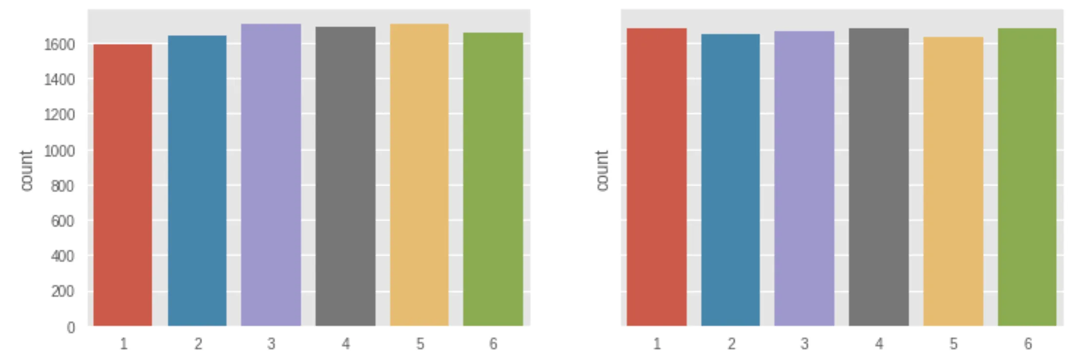
And when we look at the sums?

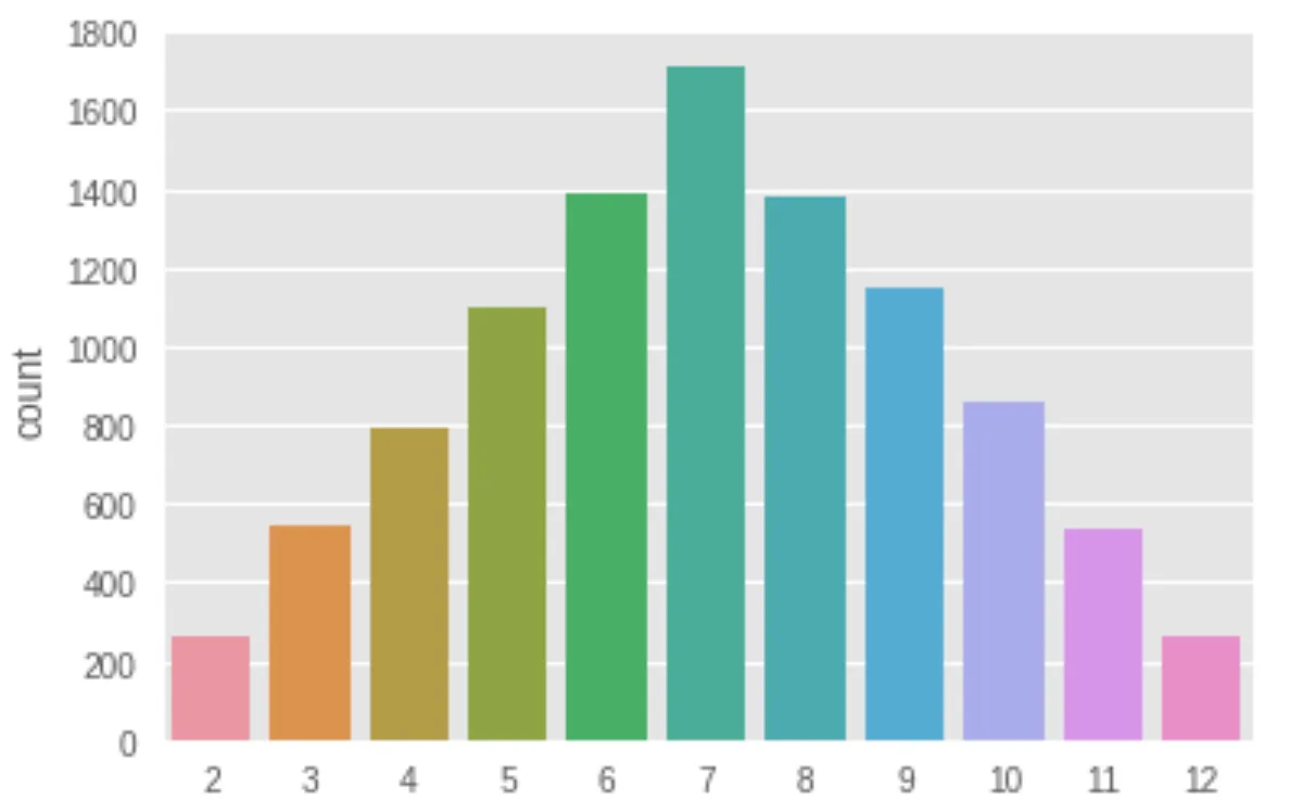
These values have also converged towards their expected outcomes, though the difference isn’t as stark.

The Rules of Craps

In craps, the main bet (Pass Line) is on whether the shooter (dice-roller) can throw the “point” number before a $7$ is rolled. The shooter starts the game by throwing $2$ dice. The sum becomes the “point” number, unless the shooter rolls a $7$ or $11$ on the come-out roll. Then everyone’s bet on the pass line wins even money. If the shooter comes out with a $2$, $3$, or $12$ — this is called craps — everyone loses their Pass Line bets.

If the shooter rolls any other number, this number becomes the point.

Every roll after that is a gamble against a seven. Players with money on the Pass Line bet are hoping the shooter will throw that number before they throw a 7.

The Odds

So how badly are the odds stacked against the shooter? Well, it doesn’t look good.

Run the following code and see for yourself:

We see percentages that back up the graphs we generated earlier. Though we determined this experimentally, it’s easy to validate our answer theoretically.

Let’s return to our discussion of probability from earlier in the post. Remember that the probability of an event occurring is equal to the number of outcomes where the event occurs divided by the number of total possible outcomes.

So what are all the possible combinations of dice rolls?

Looking at the table, we can see that there are $6$ different combinations that add up to seven. Since there are a total of $36$ possible combinations, the probability of rolling a seven is $6 / 36$, or $16.67$.

There are 5 combinations that sum to $8$, and $5$ combinations that sum to $6$. The chances of rolling either of those numbers is $5 / 36$, or $13.89$. If we calculate the probabilities for the rest of the outcomes, we can start to see why Las Vegas will always make money in the long run.

Maybe I’ll reconsider my dice-playing ways the next time I visit the casinos.

Back to the Game

So what about our game with Xochitl and Jimmie? To figure out who has the short end of the stick here, we’ll need to run some calculations.

For Xochitl, she’s betting on the sum of two dice resulting in a prime number. For Jimmie, he needs both numbers on the dice to the be the same. Let’s calculate the probability for each player winning using our experimental results.

Here’s some python to make it happen.

Now that we have the probability of each player making money, we can use that to calculate the expectation for both Jimmie and Xochitl. Wikipedia defines expected value like so:

In probability theory, the expected value of a random variable, intuitively, is the long-run average value of repetitions of the same experiment it represents. More practically, the expected value of a discrete random variable is the probability-weighted average of all possible values.

What this is saying is that we need to multiply the probability by the amount each player would earn. Doing so gives us $.16666 * 2 = .33333$ for Jimmie and $.4159 * 1 = .4159$ for Xochitl. Even though Jimmie earns 2X as much money each time he wins, it would still be advantageous to choose Xochitl’s strategy if we’re looking to make money in the long run.

Wrapping Up

My main conclusion? Odds are odds and chances are I’m going to lose all my money if I keep going back to Las Vegas. At least I know enough programming and stats to figure that out. And now you do too.

Simulating random experiments like these are a great way to get a handle on statistics that can get very math heavy. I didn’t go into distributions here, but there’s definitely more to add on to that subject when I have more time.

This concept is originally taken from an EdX - MIT Fundamentals of Statistics course that I thoroughly enjoyed and can be found here .

← Previous Post

Using CSS Grid For Landing Pages

March 11, 2019

Next Post →

Design in CSS: Colors, Fonts, and Themes

March 25, 2019